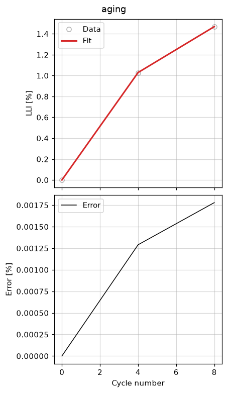
Cycle-ageing fit

Fit an SEI solvent diffusivity from cycle-ageing summary data (loss of lithium inventory vs cycle number) with CycleAgeing and DataFit.

This fits LLI [%], a built-in default metric, so it needs no metrics option. A custom metric is expressible too, as a metrics config — this one is last-minus-first of the cycle-wise discharge capacity over each cycle’s first step:

metrics = {
    "C/5 capacity [A.h]": {
        "type": "ComposedMetric",
        "operation": "sub",
        "left": {
            "type": "CyclewiseMetric",
            "step": 0,
            "metric": {"type": "Last", "variable": "Discharge capacity [A.h]"},
        },
        "right": {
            "type": "CyclewiseMetric",
            "step": 0,
            "metric": {"type": "First", "variable": "Discharge capacity [A.h]"},
        },
    }
}

The summary data below has no discharge-capacity column to compare it against, so this fit omits it.

from ionworks import Ionworks
import ionworks_schema as iws
import matplotlib.pyplot as plt
import pandas as pd
import pybamm

# Synthetic example summary, one row per RPT: Cycle number and LLI [%]. Swap in your
# own export, or read a measurement with `client.cell_measurement`.
data = pd.read_csv(iws.example_data("cycle_ageing_summary"))

# A fit needs a complete parameter set, not just the ones you know.
known = iws.direct_entries.DirectEntry(
    parameters=dict(pybamm.ParameterValues("Chen2020"))
)

# RPT: a slow C/5 discharge (the LLI read) then a rest. `experiment` also
# takes UCP: https://docs.ionworks.com/simulate/universal-cycler-protocol
rpt = [
    {
        "type": "c-rate",
        "value": 0.2,
        "terminations": [{"type": "voltage", "value": 2.5}],
        "period": 60.0,
    },
    {"type": "rest", "duration": "10 minutes"},
]
# Faster cycle that ages the cell between RPTs. Both steps are constant
# current; add a voltage step for a CV taper.
cc_cycle = [
    {
        "type": "c-rate",
        "value": 1.0,
        "terminations": [{"type": "voltage", "value": 2.5}],
    },
    {
        "type": "c-rate",
        "value": -0.5,
        "terminations": [{"type": "voltage", "value": 4.2}],
    },
]
# 3 ageing cycles + 1 RPT per block; two blocks after an initial RPT gives
# the 9 cycles matching Cycle number 0, 4 and 8 in the data.
experiment = {"cycles": [rpt] + ([cc_cycle] * 3 + [rpt]) * 2}

objectives = {
    "aging": iws.objectives.CycleAgeing(
        data=data,
        options=iws.objectives.CycleAgeingOptions(
            model=pybamm.lithium_ion.SPMe(
                options={"SEI": "solvent-diffusion limited"}
            ),
            experiment=experiment,
            objective_variables=["LLI [%]"],
            # LLI [%] is a default metric, so `metrics` can stay unset.
        ),
    )
}
# We fit the SEI solvent diffusivity.
parameters = {
    "SEI solvent diffusivity [m2.s-1]": iws.Parameter(
        "SEI solvent diffusivity [m2.s-1]",
        initial_value=5e-19,
        bounds=(1e-20, 1e-18),
    ),
}

fit = iws.DataFit(
    objectives=objectives,
    parameters=parameters,
    cost=iws.costs.RMSE(),
    # Small population and iteration count keep the example quick; a
    # harder fit needs more.
    optimizer=iws.optimizers.PSO(population_size=10, max_iterations=15),
    # PSO is stochastic; the seed makes the run reproducible.
    options=iws.DataFitOptions(seed=0),
)

client = Ionworks()
submission = client.pipeline.create(iws.Pipeline({"known": known, "aging": fit}))
client.pipeline.wait_for_completion(submission.id)
result = client.pipeline.result(submission.id)
fit_result = result.element("aging")
figs = fit_result.plot_fit_results()
plt.show()