Using callbacks in objectives

This notebook explains how to use a callback in an objective function. For details on the Callback class, see the API reference. Potential use cases for this are:

• Plotting some outputs at each iteration of the optimization

• Saving internal variables to plot once the optimization is complete

Some objectives have “internal callbacks” which are not intended to be user facing. These are standard callbacks that can be used to plot the results of an optimization by using DataFit.plot_fit_results(). For user-facing callbacks, users should create their own callback objects and call them directly for plotting, as demonstrated in this notebook.

Creating a custom callback

To implement a custom callback, create a class that inherits from iwp.callbacks.Callback and calls some specific functions. See the documentation for iwp.callbacks.Callback for more information on the available functions and their expected inputs.

import ionworkspipeline as iwp
import matplotlib.pyplot as plt
import numpy as np
import pandas as pd
import pybamm

/Users/runner/work/ionworks-app/ionworks-app/.venv/lib/python3.12/site-packages/tqdm/auto.py:21: TqdmWarning: IProgress not found. Please update jupyter and ipywidgets. See https://ipywidgets.readthedocs.io/en/stable/user_install.html
  from .autonotebook import tqdm as notebook_tqdm

class MyCallback(iwp.callbacks.Callback):
    def __init__(self):
        super().__init__()
        # Implement our own iteration counter
        self.iter = 0

    def on_objective_build(self, logs):
        self.data_ = logs["data"]

    def on_run_iteration(self, logs):
        # Print some information at each iteration
        inputs = logs["inputs"]
        V_model = logs["outputs"]["Voltage [V]"]
        V_data = self.data_["Voltage [V]"]

        # calculate RMSE, note this is not necessarily the cost function used in the optimization
        rmse = np.sqrt(np.nanmean((V_model - V_data) ** 2))

        print(f"Iteration: {self.iter}, Inputs: {inputs}, RMSE: {rmse}")
        self.iter += 1

    def on_datafit_finish(self, logs):
        self.fit_results_ = logs

    def plot_fit_results(self):
        """
        Plot the fit results.
        """
        data = self.data_
        fit = self.fit_results_["outputs"]

        fit_results = {
            "data": (data["Time [s]"], data["Voltage [V]"]),
            "fit": (fit["Time [s]"], fit["Voltage [V]"]),
        }

        markers = {"data": "o", "fit": "--"}
        colors = {"data": "k", "fit": "tab:red"}
        fig, ax = plt.subplots()
        for name, (t, V) in fit_results.items():
            ax.plot(
                t,
                V,
                markers[name],
                label=name,
                color=colors[name],
                mfc="none",
                linewidth=2,
            )
        ax.grid(alpha=0.5)
        ax.set_xlabel("Time [s]")
        ax.set_ylabel("Voltage [V]")
        ax.legend()

        return fig, ax

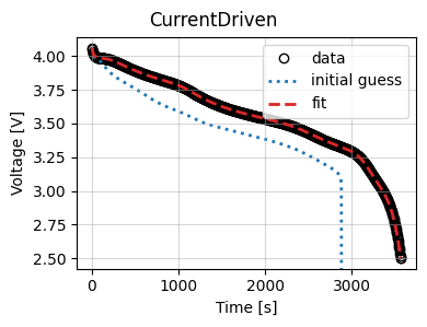
To use this callback, we generate synthetic data for a current-driven experiment and fit a SPM using the CurrentDriven objective.

model = pybamm.lithium_ion.SPM()
parameter_values = iwp.ParameterValues("Chen2020")
t = np.linspace(0, 3600, 1000)
sim = iwp.Simulation(model, parameter_values=parameter_values, t_eval=t, t_interp=t)
sim.solve()
data = pd.DataFrame(
    {x: sim.solution[x].entries for x in ["Time [s]", "Current [A]", "Voltage [V]"]}
)

# In this example we just fit the diffusivity in the positive electrode
parameters = {
    "Positive particle diffusivity [m2.s-1]": iwp.Parameter("D_s", initial_value=1e-15),
}

# Create the callback
callback = MyCallback()
objective = iwp.objectives.CurrentDriven(
    data, options={"model": model}, callbacks=callback
)
current_driven = iwp.DataFit(objective, parameters=parameters)

# make sure we're not accidentally initializing with the correct values by passing
# them in
params_for_pipeline = {k: v for k, v in parameter_values.items() if k not in parameters}

results = current_driven.run(params_for_pipeline)

Iteration: 0, Inputs: {'D_s': 1e-15}, RMSE: 41385.461471170194
Iteration: 1, Inputs: {'D_s': 1e-15}, RMSE: 41385.461471170194
Iteration: 2, Inputs: {'D_s': 2e-15}, RMSE: 0.06456358996285798
Iteration: 3, Inputs: {'D_s': 0.0}, RMSE: 9999999996.444775
Iteration: 4, Inputs: {'D_s': 1.500000000017129e-15}, RMSE: 5008.29318808216
Iteration: 5, Inputs: {'D_s': 2.2500000000000003e-15}, RMSE: 0.05121636924394488
Iteration: 6, Inputs: {'D_s': 2.1359453724793022e-15}, RMSE: 0.05695977346389743
Iteration: 7, Inputs: {'D_s': 2.3500000000000003e-15}, RMSE: 0.046577866000250545
Iteration: 8, Inputs: {'D_s': 2.2680388770594857e-15}, RMSE: 0.05035396992480285
Iteration: 9, Inputs: {'D_s': 2.4500000000000004e-15}, RMSE: 0.042264908978351654
Iteration: 10, Inputs: {'D_s': 2.359019441153719e-15}, RMSE: 0.046176143663567384
Iteration: 11, Inputs: {'D_s': 2.5000000000000004e-15}, RMSE: 0.04021917402820903
Iteration: 12, Inputs: {'D_s': 2.570710678118655e-15}, RMSE: 0.03744047833130332
Iteration: 13, Inputs: {'D_s': 2.670710678118655e-15}, RMSE: 0.03372422141962414
Iteration: 14, Inputs: {'D_s': 2.8121320343559647e-15}, RMSE: 0.028858603766024702
Iteration: 15, Inputs: {'D_s': 3.012132034355965e-15}, RMSE: 0.022634750821423192
Iteration: 16, Inputs: {'D_s': 3.294974746830584e-15}, RMSE: 0.014955406717505927
Iteration: 17, Inputs: {'D_s': 3.577025556232543e-15}, RMSE: 0.008352003871117222
Iteration: 18, Inputs: {'D_s': 3.76052758604426e-15}, RMSE: 0.004525399886297545
Iteration: 19, Inputs: {'D_s': 3.8943250897936825e-15}, RMSE: 0.0019367143930845102

Iteration: 20, Inputs: {'D_s': 3.965646359449817e-15}, RMSE: 0.0006202840859151885
Iteration: 21, Inputs: {'D_s': 3.992177245746258e-15}, RMSE: 0.00014141620239612764
Iteration: 22, Inputs: {'D_s': 3.999021987945655e-15}, RMSE: 2.0033329988651146e-05
Iteration: 23, Inputs: {'D_s': 4.009021987945655e-15}, RMSE: 0.00016017064913520366
Iteration: 24, Inputs: {'D_s': 4.000074780279531e-15}, RMSE: 7.575066333595016e-06
Iteration: 25, Inputs: {'D_s': 4.001074780279531e-15}, RMSE: 1.9681163769159943e-05
Iteration: 26, Inputs: {'D_s': 3.999974780279531e-15}, RMSE: 7.717392575579396e-06
Iteration: 27, Inputs: {'D_s': 4.000174780279531e-15}, RMSE: 7.84874506893488e-06
Iteration: 28, Inputs: {'D_s': 4.000058800669547e-15}, RMSE: 7.569671456308183e-06
Iteration: 29, Inputs: {'D_s': 4.0000488006695475e-15}, RMSE: 7.571783281249286e-06
Iteration: 30, Inputs: {'D_s': 4.000059800669547e-15}, RMSE: 7.569692672696082e-06
Iteration: 31, Inputs: {'D_s': 4.000057800669547e-15}, RMSE: 7.569692498806178e-06
Iteration: 32, Inputs: {'D_s': 4.000058800669547e-15}, RMSE: 7.569671456308183e-06

Now we use the results to plot the fit at the end of the optimization.

_ = results.plot_fit_results()

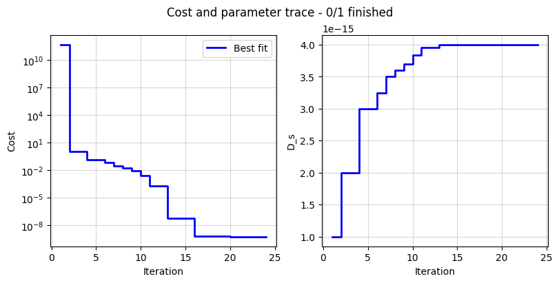
Cost logger

The DataFit class has an internal “cost-logger” attribute that can be used to log and visualize the cost function during optimization. This is useful for monitoring the progress of the optimization. The cost logger is a dictionary that stores the cost function value at each iteration. The cost logger can be accessed using the cost_logger attribute of the DataFit object.

By default, the cost logger tracks the cost function value. DataFit.plot_trace can be used the plot the progress at the end of the optimization.

objective = iwp.objectives.CurrentDriven(data, options={"model": model})
current_driven = iwp.DataFit(objective, parameters=parameters)
_ = current_driven.run(params_for_pipeline)
_ = current_driven.plot_trace()

The cost logger can be changed by passing the cost_logger argument to the DataFit object. For example, the following example shows how to pass a cost logger that plots the cost function and parameter values every 10 seconds.

current_driven = iwp.DataFit(
    objective,
    parameters=parameters,
    cost_logger=iwp.CostLogger(plot_every=10),
)