Cycle ageing example

This notebook demonstrates how to use the CycleAgeing objective function to fit the SEI solvent diffusivity in the “solvent-diffusion limited” SEI model using synthetic cycling data.

import ionworkspipeline as iwp
from ionworkspipeline.data_fits.models.metrics import First, Last
import matplotlib.pyplot as plt
import numpy as np
import pandas as pd
import pybamm

We begin by generating some synthetic cycling data. We choose the SPMe model and the “solvent-diffusion limited” SEI model and simulate CCCV charge/discharge cycling with RPTs every 10 cycles. For the data, we record the cycle number, the loss of lithium inventory, and the C/5 discharge capacity. We choose the parameter values so that we get a large loss of lithium inventory even after only 50 cycles.

# Model and parameters
model = pybamm.lithium_ion.SPMe({"SEI": "solvent-diffusion limited"})
parameter_values = pybamm.ParameterValues("Chen2020")
parameter_values.update({"SEI solvent diffusivity [m2.s-1]": 5e-19})

# Define RPT and CCCV cycles
rpt_cycle = (
    "Discharge at C/5 until 2.5 V (60s period)",
    "Rest for 1 hour",
    "Charge at C/5 until 4.2 V",
    "Hold at 4.2 V until 10 mA",
    "Rest for 1 hour",
)
cccv_cycle = (
    "Discharge at 1C until 2.5 V",
    "Rest for 1 hour",
    "Charge at C/2 until 4.2 V",
    "Hold at 4.2 V until 10 mA",
    "Rest for 1 hour",
)
# One block = 10 CCCV cycles + 1 RPT
one_block = [cccv_cycle] * 10 + [rpt_cycle]
# Simulate initial RPT, then 10 CCCV cycles + 1 RPT repeated 5 times
cycles_list = [rpt_cycle] + one_block * 5
experiment = pybamm.Experiment(cycles_list)
sim = pybamm.Simulation(model, experiment=experiment, parameter_values=parameter_values)
sol = sim.solve()

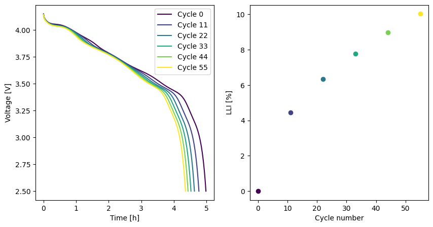
We can extract the synthetic data from the simulation and plot the RPTs to observe the effect of the degradation

# Indices of cycles that are RPTs (0, 11, 21, ..., as RPT cycles are every 11 cycles)
rpt_idxs = np.arange(0, len(cycles_list), 11)

# Extract the data and plot the RPTs
data_rows = []
fig, ax = plt.subplots(1, 2, figsize=(10, 5))
ax[0].set_xlabel("Time [h]")
ax[0].set_ylabel("Voltage [V]")
ax[1].set_xlabel("Cycle number")
ax[1].set_ylabel("LLI [%]")
colors = plt.cm.viridis(np.linspace(0, 1, len(rpt_idxs)))
for idx, color in zip(rpt_idxs, colors, strict=False):
    # Extract the cycle solution and the C/5 discharge step
    cycle_sol = sol.cycles[idx]
    step_sol = cycle_sol.steps[0]

    # Store LLI
    LLI = cycle_sol["LLI [%]"].data[0]
    # Calculate C/5 discharge capacity
    q = step_sol["Discharge capacity [A.h]"].data
    q_c5 = q[-1] - q[0]
    data_rows.append(
        {
            "Cycle number": idx,
            "LLI [%]": LLI,
            "C/5 capacity [A.h]": q_c5,
        }
    )

    # Plot C/5 discharge from RPT and LLI
    time = step_sol["Time [h]"].data
    time -= time[0]
    voltage = step_sol["Voltage [V]"].data
    ax[0].plot(time, voltage, color=color, label=f"Cycle {idx}")
    ax[1].scatter(idx, LLI, color=color)

ax[0].legend()

# Convert to DataFrame
data = pd.DataFrame(data_rows)

Next, we create the objective function. We pass the data and the options to the CycleAgeing objective function. The options include the model, experiment, the objective variables (i.e. the variables we want to fit to), and the metrics that define how to extract values from the simulation.

The metrics option accepts a dictionary mapping variable names to Metric objects. We can combine metrics to create new metrics, which enables calculating more complex quantities that aren’t directly in the model, such as the C/5 discharge capacity or the pulse resistance. Here we use First("LLI [%]").by_cycle() to extract the first value of the loss of lithium inventory at each cycle and use the Last("Discharge capacity [A.h]").by_cycle(step=0) - First("Discharge capacity [A.h]").by_cycle(step=0) to extract the C/5 discharge capacity at each cycle. The .by_cycle() method evaluates the metric for each cycle in the simulation. We pass the step=0 argument to the by_cycle() method to extract the values from the first step of the cycle.

objective = iwp.objectives.CycleAgeing(
    data,
    options={
        "model": model,
        "experiment": experiment,
        "objective variables": ["LLI [%]", "C/5 capacity [A.h]"],
        "metrics": {
            "LLI [%]": First("LLI [%]").by_cycle(),
            "C/5 capacity [A.h]": Last("Discharge capacity [A.h]").by_cycle(step=0)
            - First("Discharge capacity [A.h]").by_cycle(step=0),
        },
    },
)

We then create the data fit. We pass the objective function and the parameters to the DataFit class. The parameters include the initial values and bounds for the parameters we want to fit.

parameters = {
    "SEI solvent diffusivity [m2.s-1]": iwp.Parameter(
        "SEI solvent diffusivity [m2.s-1]",
        bounds=(1e-20, 1e-18),
    )
}
optimizer = iwp.optimizers.Pints(method="PSO", log_to_screen=True)
data_fit = iwp.DataFit(objective, parameters=parameters)

Next, we run the data fit. We pass the known parameters (i.e. those we are not fitting) to the data fit.

known_parameters = {k: v for k, v in parameter_values.items() if k not in parameters}
data_fit.run(known_parameters)

Result(
  SEI solvent diffusivity [m2.s-1]: 5e-19
)

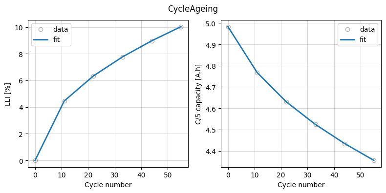
Finally, we plot the fit results.

_ = data_fit.plot_fit_results()

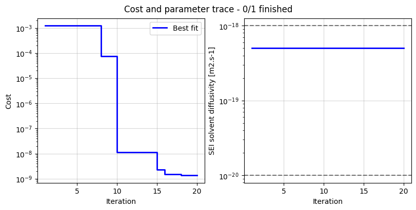
data_fit.plot_trace()

(<Figure size 800x400 with 2 Axes>,
 array([<Axes: xlabel='Iteration', ylabel='Cost'>,
        <Axes: xlabel='Iteration', ylabel='SEI solvent diffusivity [m2.s-1]'>],
       dtype=object))