Fitting electrolyte conductivity (Landesfeind 2019 form)

Landesfeind & Gasteiger (2019) report measurements of the four binary-electrolyte transport properties — ionic conductivity \(\kappa\), salt diffusion coefficient \(D_e\), thermodynamic factor \(\chi\) and cation transference number \(t_+^0\) — for three solvent systems (EC:DMC (1:1), EC:EMC (3:7), EMC:FEC (19:1)) over a wide \((c_e, T)\) range, and provide a closed-form fit for each property. For the ionic conductivity (in mS/cm, with \(c\) in mol/L and \(T\) in K) the closed form is

\[\kappa(c, T) = \underbrace{p_1\,(1 + (T - p_2))}_{A(T)}\;c\; \frac{\overbrace{1 + p_3\,\sqrt{c} + p_4\,(1 + p_5\,e^{1000/T})\,c}^{B(c,T)}} {\underbrace{1 + p_6\,e^{1000/T}\,c^{4}}_{C(c,T)}}\,,\]

with six fitted coefficients \(p_1, \dots, p_6\) per solvent system. (The diffusivity, TDF and transference number have analogous closed forms with their own coefficients — 4, 9 and 9 respectively.)

iwp.direct_entries.landesfeind_electrolyte(c_e, system) packages all four functions plus the published coefficients for the chosen system as a single DirectEntry. Critically, the coefficients are stored as pybamm.Parameters rather than hard-coded numbers, which means we can override any of them with iwp.Parameter in a pipeline to refit them to our own data — without reimplementing the closed form. This notebook demonstrates that workflow on the conductivity coefficients.

We work at a single isotherm (\(T = 293.15\) K, the closest measurement temperature in Landesfeind 2019 to \(25\) °C). We compare three things:

1. Digitized paper data at \(T = 293.15\) K, plotted against the published equation (no fit — the published \(p_1\dots p_6\) are already in the direct entry).

2. Mock data generated from the published equation at \(T = 293.15\) K with added Gaussian noise.

3. A fit to the mock data, recovering a subset of the published coefficients.

At a single \(T\) the six coefficients are not all separately identifiable: \(p_2\) enters only via the prefactor \(A(T) = p_1\,(1 + (T - p_2))\) and is perfectly correlated with \(p_1\) when \(T\) is fixed; likewise the temperature-coupled terms \(p_5\,e^{1000/T}\) and \(p_6\,e^{1000/T}\) collapse to constants. We therefore hold \(p_2\), \(p_5\), \(p_6\) at their published values and fit the remaining three (\(p_1\), \(p_3\), \(p_4\)).

import ionworkspipeline as iwp
import matplotlib.pyplot as plt
import numpy as np
import pandas as pd
import pybamm

/Users/runner/work/ionworks-app/ionworks-app/.venv/lib/python3.12/site-packages/tqdm/auto.py:21: TqdmWarning: IProgress not found. Please update jupyter and ipywidgets. See https://ipywidgets.readthedocs.io/en/stable/user_install.html
  from .autonotebook import tqdm as notebook_tqdm

1. The Landesfeind direct entry

landesfeind_electrolyte returns a DirectEntry whose parameters dict contains the conductivity, diffusivity, TDF and transference number functions, plus the published numeric values for every coefficient those functions reference. We grab the conductivity function — which still has \(p_1, \dots, p_6\) as pybamm.Parameters — so we can evaluate it later with the published coefficients (for reference curves) and inside the fitting objective (with \(p_1, p_3, p_4\) replaced by InputParameters the optimizer sets).

electrolyte_entry = iwp.direct_entries.landesfeind_electrolyte(
    c_e=1000, system="EC:EMC (3:7)"
)
kappa_func = electrolyte_entry.parameters["Electrolyte conductivity [S.m-1]"]

2. Digitized paper data at \(T = 293.15\) K

The CSV landesfeind_2019_ec_emc_3_7.csv was sourced from the CALiSol-23 dataset, which digitized the conductivity points from the figures of Landesfeind & Gasteiger 2019. We filter to the \(T = 293.15\) K isotherm.

all_paper_data = pd.read_csv("landesfeind_2019_ec_emc_3_7.csv")
T_iso = 293.15  # K
paper_data = all_paper_data[all_paper_data["Temperature [K]"] == T_iso].reset_index(
    drop=True
)
paper_data

	Electrolyte concentration [mol.m-3]	Temperature [K]	Electrolyte conductivity [S.m-1]
0	102.0	293.15	0.2467
1	497.0	293.15	0.6796
2	998.0	293.15	0.8267
3	1499.0	293.15	0.7172
4	2003.0	293.15	0.5047
5	3000.0	293.15	0.2216

3. Generate mock data

We sample the published equation on a denser concentration grid at the same temperature and add 5% Gaussian noise. This is what a clean experimental campaign at this isotherm might produce.

rng = np.random.default_rng(0)
c_mock = np.linspace(100, 3000, 12)  # mol/m^3
T_mock = np.full_like(c_mock, T_iso)

c_vec = pybamm.Vector(c_mock[:, np.newaxis])
T_vec = pybamm.Vector(T_mock[:, np.newaxis])
kappa_published = (
    iwp.ParameterValues(electrolyte_entry.parameters)
    .process_symbol(kappa_func(c_vec, T_vec))
    .evaluate()
    .flatten()
)
kappa_mock = kappa_published * (1 + 0.05 * rng.standard_normal(c_mock.size))
mock_data = pd.DataFrame(
    {
        "Electrolyte concentration [mol.m-3]": c_mock,
        "Temperature [K]": T_mock,
        "Electrolyte conductivity [S.m-1]": kappa_mock,
    }
)
mock_data.head()

	Electrolyte concentration [mol.m-3]	Temperature [K]	Electrolyte conductivity [S.m-1]
0	100.000000	293.15	0.241467
1	363.636364	293.15	0.591138
2	627.272727	293.15	0.792801
3	890.909091	293.15	0.839785
4	1154.545455	293.15	0.804313

4. A custom fitting objective

Because we are fitting an algebraic relationship rather than a PyBaMM simulation, we subclass FittingObjective and skip the simulation in build. The conductivity function is taken straight from all_parameter_values (which the pipeline populates from the direct entry) — we don’t reimplement the equation. We bake the data points \((c_e, T)\) into the symbol as pybamm.Vectors once in build, so each optimizer step is a single vectorized evaluate rather than a Python loop. The fitted coefficients \(p_1, p_3, p_4\) remain InputParameters that the optimizer feeds in via the inputs dict.

class LandesfeindConductivityObjective(iwp.objectives.FittingObjective):
    def process_data(self):
        data = self.data["data"]
        self._processed_data = {
            "Electrolyte conductivity [S.m-1]": data[
                "Electrolyte conductivity [S.m-1]"
            ].values
        }

    def build(self, all_parameter_values):
        data = self.data["data"]
        c_e = data["Electrolyte concentration [mol.m-3]"].values[:, np.newaxis]
        T = data["Temperature [K]"].values[:, np.newaxis]
        kappa = all_parameter_values["Electrolyte conductivity [S.m-1]"]
        self._processed_kappa = all_parameter_values.process_symbol(
            kappa(pybamm.Vector(c_e), pybamm.Vector(T))
        )

    def run(self, inputs, full_output=False):
        return {
            "Electrolyte conductivity [S.m-1]": self._processed_kappa.evaluate(
                inputs=inputs
            ).flatten()
        }

5. Fit \(p_1\), \(p_3\), \(p_4\) to the mock data

The fit parameters use the same names as the coefficients defined inside landesfeind_electrolyte, so the pipeline replaces them with InputParameters while leaving \(p_2\), \(p_5\), \(p_6\) at the published values from the direct entry.

fit_parameters = {
    name: iwp.Parameter(name, initial_value=v0, bounds=bnds)
    for name, v0, bnds in [
        ("Landesfeind electrolyte conductivity p1", 0.3, (1e-3, 5)),
        ("Landesfeind electrolyte conductivity p3", -0.5, (-5, 5)),
        ("Landesfeind electrolyte conductivity p4", 0.5, (-2, 2)),
    ]
}

objective = LandesfeindConductivityObjective(mock_data)
datafit = iwp.DataFit(objective, parameters=fit_parameters)

pipeline = iwp.Pipeline(
    {
        "electrolyte": electrolyte_entry,
        "fit": datafit,
    }
)
fitted_values = pipeline.run()

Compare fitted vs published values:

comparison = pd.DataFrame(
    {
        "published": [electrolyte_entry.parameters[name] for name in fit_parameters],
        "fit (mock data)": [fitted_values[name] for name in fit_parameters],
    },
    index=list(fit_parameters),
)
comparison

	published	fit (mock data)
Landesfeind electrolyte conductivity p1	0.521	0.511212
Landesfeind electrolyte conductivity p3	-1.060	-1.038286
Landesfeind electrolyte conductivity p4	0.353	0.338020

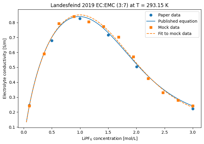
6. Plot at \(T = 293.15\) K

We plot, on the same axes:

• The 6 digitized paper data points and the published equation curve (no fit — taken straight from the direct entry).

• The 12 mock data points and the curve produced by the fit (\(p_1\), \(p_3\), \(p_4\) from the optimizer; \(p_2\), \(p_5\), \(p_6\) from the direct entry’s published values).

c_plot = np.linspace(50, 3000, 200)
c_vec = pybamm.Vector(c_plot[:, np.newaxis])
T_vec = pybamm.Vector(np.full_like(c_plot, T_iso)[:, np.newaxis])
sym = kappa_func(c_vec, T_vec)
published_curve = (
    iwp.ParameterValues(electrolyte_entry.parameters)
    .process_symbol(sym)
    .evaluate()
    .flatten()
)
fitted_curve = fitted_values.process_symbol(sym).evaluate().flatten()

fig, ax = plt.subplots(figsize=(7, 5))
ax.plot(
    paper_data["Electrolyte concentration [mol.m-3]"] / 1000,
    paper_data["Electrolyte conductivity [S.m-1]"],
    "o",
    color="C0",
    label="Paper data",
)
ax.plot(c_plot / 1000, published_curve, "-", color="C0", label="Published equation")
ax.plot(
    mock_data["Electrolyte concentration [mol.m-3]"] / 1000,
    mock_data["Electrolyte conductivity [S.m-1]"],
    "s",
    color="C1",
    label="Mock data",
)
ax.plot(c_plot / 1000, fitted_curve, "--", color="C1", label="Fit to mock data")
ax.set_xlabel("LiPF$_6$ concentration [mol/L]")
ax.set_ylabel("Electrolyte conductivity [S/m]")
ax.set_title(f"Landesfeind 2019 EC:EMC (3:7) at T = {T_iso} K")
ax.legend()
fig.tight_layout()