2. Full-cell OCV

In this example, we use synthetic full-cell GITT data and known half-cell OCP parameters to determine the stoichiometry windows that give the correct full-cell OCV, a process often referred to as “electrode balancing”.

Before running this example, make sure to run the script true_parameters/generate_data.py to generate the synthetic data.

from pathlib import Path

import ionworkspipeline as iwp
import iwutil
from true_parameters.parameters import get_msmr_parameters

Cell balancing theory

Given the open-circuit potentials for each electrode, we combine them to get the full-cell open-circuit voltage

\[U_{cell}(z) = U_{p}(\theta_{p}) - U_{n}(\theta_{n}),\]

where \(z\) is the full-cell state of charge, and \(\theta_{n}\) and \(\theta_{p}\) are the electrode-level state of charge of the negative and positive electrodes respectively (usually called “stoichiometry” or “lithiation” to avoid confusion with cell-level state of charge). To evaluate the OCV, we need to convert the stoichiometry of each electrode to the full-cell state of charge. This is done using the following formula:

\[ z = \frac{\theta_{n} - \theta_{n}^\mathrm{0}}{\theta_{n}^\mathrm{100} - \theta_{n}^\mathrm{0}} = \frac{\theta_{p} - \theta_{p}^\mathrm{0}}{\theta_{p}^\mathrm{100} - \theta_{p}^\mathrm{0}}, \]

where \(\theta_{n}^\mathrm{0}\), \(\theta_{n}^\mathrm{100}\), \(\theta_{p}^\mathrm{0}\), \(\theta_{p}^\mathrm{100}\) are the stoichiometries of the negative and positive electrodes at 0% and 100% state of charge respectively. Hence the challenge is to find the four values \(\theta_{n}^\mathrm{0}\), \(\theta_{n}^\mathrm{100}\), \(\theta_{p}^\mathrm{0}\), \(\theta_{p}^\mathrm{100}\), that best fit the full-cell open-circuit voltage data. In practice, full-cell OCV data is is given in terms of capacity instead of stoichiometry. Therefore, we reformulate the full-cell open-circuit voltage as a function of capacity:

\[U_{cell}(q) = U_{p}(q_{p}) - U_{n}(q_{n}),\]

where \(q = Qz\), \(q_{n} = \theta_{n}Q_{n}\), \(q_{p} = \theta_{p}Q_{p}\), and \(Q\) is the total capacity of the cell and \(Q_{n}\) and \(Q_{p}\) are the total capacities of the individual electrodes. We can then convert between the full-cell capacity and the electrode capacities using the following formula:

\[ q/Q = \frac{q_{n} - q_{n}^\mathrm{0}}{q_{n}^\mathrm{100} - q_{n}^\mathrm{0}} = \frac{q_{p} - q_{p}^\mathrm{0}}{q_{p}^\mathrm{100} - q_{p}^\mathrm{0}}. \]

We find the values of \(q_{n}^\mathrm{0}\), \(q_{n}^\mathrm{100}\), \(q_{p}^\mathrm{0}\), \(q_{p}^\mathrm{100}\) that best fit the data.

In this example, we fit the “lower excess capacity” and “upper excess capacity” instead of the stoichiometries at 0% and 100% state of charge. We use these names because the data typically does not reach the true 0% and 100% state of charge, due to kinetic limitations and/or electrolyte stability. The lower excess capacity is equal to \(q_{n}^\mathrm{0}\) in the negative electrode, and \(q_{p}^\mathrm{100}\) in the positive electrode. The upper excess capacity is equal to \(Q_{n} - q_{n}^\mathrm{100}\) in the negative electrode, and \(Q_{p} - q_{p}^\mathrm{0}\) in the positive electrode. \(Q\) is given by the actual total capacity observed in the experimental data (called “useable capacity” in the example).

Load the data

We load the synthetic GITT data and the extract the OCP from the relaxed voltages.

gitt_data = iwutil.read_df(Path("synthetic_data") / "full_cell" / "gitt.csv")
ocp_data = iwp.data_fits.preprocess.pulse_data_to_ocp(gitt_data)

Get the known parameters

In this example, we assume we already know the MSMR OCP parameters for the negative and positive electrodes. In practice, these parameters can be fitted using the half-cell OCV workflow.

msmr_params_n = get_msmr_parameters("negative")
msmr_params_p = get_msmr_parameters("positive")
known_params = {
    **msmr_params_n,
    **msmr_params_p,
    "Ambient temperature [K]": 298.15,
}

Set up the parameters to fit

Now we set up our initial guesses for the parameters. As in the previous example, we create a dictionary of Parameter objects.

Q_use = ocp_data["Capacity [A.h]"].max()
Q_n_lowex = iwp.Parameter(
    "Q_n_lowex", initial_value=0.01 * Q_use, bounds=(0, 0.2 * Q_use)
)
Q_p_lowex = iwp.Parameter("Q_p_lowex", initial_value=0.1 * Q_use, bounds=(0, Q_use))
Q_n_uppex = iwp.Parameter(
    "Q_n_uppex", initial_value=0.1 * Q_use, bounds=(0, 0.2 * Q_use)
)
Q_p_uppex = iwp.Parameter("Q_p_uppex", initial_value=0.5 * Q_use, bounds=(0, Q_use))
parameters = {
    "Negative electrode lower excess capacity [A.h]": Q_n_lowex,
    "Positive electrode lower excess capacity [A.h]": Q_p_lowex,
    "Negative electrode upper excess capacity [A.h]": Q_n_uppex,
    "Positive electrode upper excess capacity [A.h]": Q_p_uppex,
    "Negative electrode capacity [A.h]": Q_n_lowex + Q_use + Q_n_uppex,
    "Positive electrode capacity [A.h]": Q_p_lowex + Q_use + Q_p_uppex,
    "Usable capacity [A.h]": Q_use,
}

Run the fit

Now we are ready to run the fit. We create the objective, the DataFit object, and run the fit.

First, we create the MSMRFullCell objective function and pass in the data. We need to specify the voltage range of each electrode to use in the fit. The limits are used to evaluate the half-cell OCPs in the fit, and should therefore span a wider half-cell voltage range than we expect to see in the data.

Next, we create the DataFit object and pass in the objective and the parameters to fit. We can also customize the fitting process by passing in a cost function and selecting an optimizer.

# Create the objective
objective = iwp.objectives.MSMRFullCell(
    ocp_data,
    options={
        # these are the voltage ranges over which to evaluate the half-cell OCP curves
        "negative voltage limits": (0, 2),
        "positive voltage limits": (2.5, 5),
    },
)

# Create the DataFit object and run the fit
optimizer = iwp.optimizers.ScipyLeastSquares()
datafit = iwp.DataFit(objective, parameters=parameters, optimizer=optimizer)
results = datafit.run(known_params)

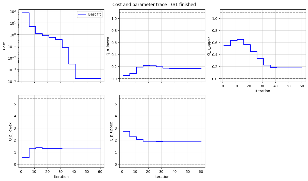
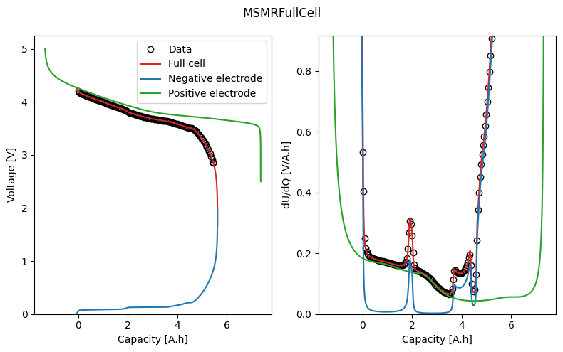
We can plot the trace of the cost function and parameter values during the fit, and the fitted OCV and dU/dQ curves. In the plot, we can see how the half-cell OCPs combine to give the full-cell OCV.

_ = datafit.plot_trace()
_ = datafit.plot_fit_results()

We can take a look at the fitted parameters by accessing the parameter_values attribute of the results object.

results.parameter_values

{'Negative electrode lower excess capacity [A.h]': 0.17026523405248983,
 'Positive electrode lower excess capacity [A.h]': 1.3504668852089856,
 'Negative electrode upper excess capacity [A.h]': 0.19325700542079832,
 'Positive electrode upper excess capacity [A.h]': 1.9147864850370082,
 'Negative electrode capacity [A.h]': 5.827846662556339,
 'Positive electrode capacity [A.h]': 8.729577793329046,
 'Usable capacity [A.h]': 5.464324423083051}