Parallelization

A DataFit evaluates its objectives on a pool of worker processes. This example shows how to choose the size of that pool, how the size you ask for relates to the size you get, and when a pool is worth having at all.

Parallelism is a property of how a fit runs, not of the fit itself, so it is configured with an ExecutionConfig passed to run rather than with a keyword on DataFit.

import time

import ionworkspipeline as iwp
from ionworkspipeline.execution import (
    ExecutionConfig,
    PrintSink,
    default_local_workers,
)
import matplotlib.pyplot as plt
import numpy as np
import pandas as pd
import pybamm

/Users/runner/work/ionworks-app/ionworks-app/.venv/lib/python3.13/site-packages/tqdm/auto.py:21: TqdmWarning: IProgress not found. Please update jupyter and ipywidgets. See https://ipywidgets.readthedocs.io/en/stable/user_install.html
  from .autonotebook import tqdm as notebook_tqdm

Setting up a fit worth parallelizing

We fit two active material volume fractions of a DFN against three discharge curves. Three objectives and an expensive model is a shape where a worker pool can actually help — we will measure how much, and see the conditions under which it does not.

First, synthetic data at three C-rates.

model = pybamm.lithium_ion.DFN()
parameter_values = iwp.ParameterValues("Chen2020")
parameter_values.update(
    {
        "Negative electrode active material volume fraction": 0.75,
        "Positive electrode active material volume fraction": 0.665,
    }
)

C_RATES = (0.2, 0.5, 1.0)


def generate_data(c_rate):
    values = parameter_values.copy()
    values["Current function [A]"] = c_rate * 5.0
    duration = 3300 / c_rate
    t = np.arange(0, duration, duration / 300)
    sim = iwp.Simulation(
        model, parameter_values=values, t_eval=[0, duration], t_interp=t
    )
    sol = sim.solve()
    return pd.DataFrame(
        {x: sol[x](sol.t) for x in ["Time [s]", "Current [A]", "Voltage [V]"]}
    )


objectives = {
    f"{c_rate}C": iwp.objectives.CurrentDriven(
        generate_data(c_rate), options={"model": model}
    )
    for c_rate in C_RATES
}

We fit with CMA-ES, a population optimizer: each iteration proposes a whole generation of candidate points, and every point in that generation can be evaluated at the same time. That is what makes a fit worth parallelizing — a optimizer that produces one point at a time can only ever occupy one worker per start, however large the pool.

Bounds are kept tight around the true values so every sampled point is a real solve rather than a cheap failure, which keeps the timings below comparable.

parameters = {
    "Negative electrode active material volume fraction": iwp.Parameter(
        "Negative electrode active material volume fraction", bounds=(0.70, 0.80)
    ),
    "Positive electrode active material volume fraction": iwp.Parameter(
        "Positive electrode active material volume fraction", bounds=(0.62, 0.72)
    ),
}
known_parameters = {k: v for k, v in parameter_values.items() if k not in parameters}


def build_data_fit(multistarts=10):
    return iwp.DataFit(
        objectives,
        parameters=parameters,
        multistarts=multistarts,
        options={"seed": 0},
        optimizer=iwp.optimizers.CMAES(population_size=8, max_iterations=15),
    )

How many workers can this fit use?

Asking for more workers than the fit can occupy does not make it faster — the extra processes sit idle. max_useful_workers() reports that ceiling, and tasks_per_point() reports how a single parameter vector fans out.

The pool is sized to min(max_useful_workers(), num_workers), so these two numbers tell you the largest num_workers worth requesting.

data_fit = build_data_fit()
data_fit.setup(known_parameters)

print(f"multistarts:          {data_fit.num_jobs}")
print(f"tasks per point:      {data_fit.tasks_per_point()}")
print(f"max useful workers:   {data_fit.max_useful_workers()}")
print(f"default pool on this machine: {default_local_workers()}")

multistarts:          10
tasks per point:      3
max useful workers:   240
default pool on this machine: 1

tasks_per_point is 3 because each parameter vector is scored against three objectives, and those solves are independent, so they are dispatched as separate tasks. max_useful_workers multiplies that fan-out by the width of one round of the search: multistarts x population_size x tasks_per_point, or 10 x 8 x 3 = 240 here. Beyond that the fit has no work to hand out.

The default pool is a fraction of the machine’s cores rather than all of them, so a fit started from an interactive session leaves the machine usable.

What one evaluation costs

Before timing the pool, it is worth knowing what it is dividing. The first evaluation in a process pays the model build and solver compile; every subsequent one is just a solve. Timing both on the freshly set-up fit shows the gap.

This has to be measured now, before any fit has run — the compiled model is cached for the lifetime of the process, so a “cold” call made later is not cold.

x0 = np.array(data_fit.x_initial_values_list)

start = time.perf_counter()
data_fit.objective_function(x0)
cold = time.perf_counter() - start

# A nearby, distinct point — the objective caches on exact inputs, so re-running
# x0 would report a cache hit rather than a solve.
start = time.perf_counter()
data_fit.objective_function(x0 * 1.001)
warm = time.perf_counter() - start

print(f"cold evaluation (build + solve): {cold:.3f}s")
print(f"warm evaluation (solve only):    {warm:.3f}s")
print(f"ratio: {cold / warm:.0f}x")

cold evaluation (build + solve): 79.676s
warm evaluation (solve only):    0.046s
ratio: 1731x

Each worker pays that build cost once. A pool of N workers therefore only wins when the warm work it removes exceeds N builds plus process startup — which is why a cheap objective (an analytic model, or a short ODE solve) usually runs slower on a local pool than in-process. The expensive model here is what makes the pool worth starting.

Choosing the worker count

Pass num_workers on an ExecutionConfig. This is the only knob needed for local execution: the pool, the in-flight task limit and the choice of executor are all derived from it.

def time_fit(num_workers):
    fit = build_data_fit()
    start = time.perf_counter()
    result = fit.run(
        known_parameters, execution=ExecutionConfig(num_workers=num_workers)
    )
    return time.perf_counter() - start, float(np.min(np.atleast_1d(result.costs)))


worker_counts = [1, 4, 8]
results = {n: time_fit(n) for n in worker_counts}
timings = {n: seconds for n, (seconds, _) in results.items()}

baseline = timings[worker_counts[0]]
for n, (seconds, cost) in results.items():
    print(
        f"num_workers={n:>2}: {seconds:6.1f}s  ({baseline / seconds:.1f}x)  cost={cost:.4e}"
    )

num_workers= 1:   60.6s  (1.0x)  cost=5.3821e-08
num_workers= 4:   28.5s  (2.1x)  cost=5.3821e-08
num_workers= 8:  103.1s  (0.6x)  cost=5.3821e-08

fig, ax = plt.subplots()
ax.plot(list(timings), list(timings.values()), "o-")
ax.set_xlabel("num_workers")
ax.set_ylabel("Fit wall time [s]")
ax.set_ylim(bottom=0)
ax.grid(alpha=0.3)

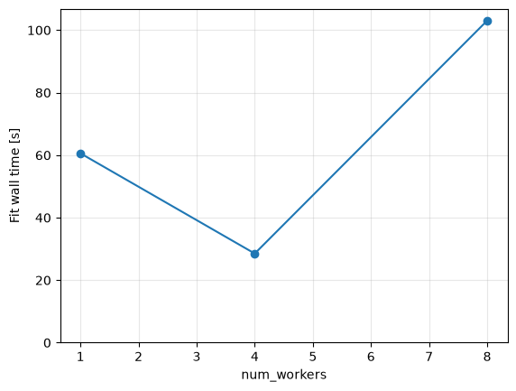
The speedup is real but sub-linear, and it flattens well before max_useful_workers. Two costs explain the gap, and both are worth knowing before choosing a number:

• Each worker builds the model once. The pool ships the objectives to every process, and the first solve in each pays the model build and solver compile.

• The pool is bounded by physical cores. Requesting more workers than the machine has oversubscribes it, and the curve turns back up.

So the useful range is roughly “up to the core count, and no more than max_useful_workers()”. Note that the fitted cost is identical at every worker count: the pool changes how fast the search runs, never what it finds.

Watching a parallel fit make progress

A print inside an objective is useless once a pool is running: it executes in a worker process, whose standard output is discarded. Progress has to come from the driver instead, and that is what a progress sink is for.

PrintSink is the built-in one — a line per generation, and a line when the fit finishes.

fit = build_data_fit(multistarts=2)
fit.run(
    known_parameters,
    execution=ExecutionConfig(num_workers=4, progress_sink=PrintSink()),
)
fig, axes = fit.plot_trace()

[0] gen    1  best 4.059720e-02

[0] gen    2  best 4.059720e-02

[0] gen    3  best 3.617948e-02

[0] gen    4  best 1.122001e-03

[1] gen    1  best 1.117309e-01

[0] gen    5  best 1.122001e-03

[1] gen    2  best 7.122784e-02

[0] gen    6  best 1.122001e-03

[1] gen    3  best 6.042567e-02

[0] gen    7  best 1.122001e-03

[1] gen    4  best 6.042567e-02

[0] gen    8  best 5.750357e-04

[1] gen    5  best 2.888953e-02

[0] gen    9  best 5.750357e-04

[1] gen    6  best 2.888953e-02

[0] gen   10  best 1.041060e-04

[1] gen    7  best 1.993269e-02

[0] gen   11  best 1.041060e-04

[1] gen    8  best 1.993269e-02

[0] gen   12  best 1.338691e-05

[1] gen    9  best 7.442355e-03

[0] gen   13  best 1.338691e-05

[1] gen   10  best 1.668895e-03

[0] gen   14  best 1.338691e-05

[1] gen   11  best 1.668895e-03

[0] gen   15  best 1.338691e-05

[1] gen   12  best 1.668895e-03

[1] gen   13  best 3.798831e-04

[1] gen   14  best 2.969829e-04

[1] gen   15  best 1.920832e-05

[1] done, best 3.884363e-06

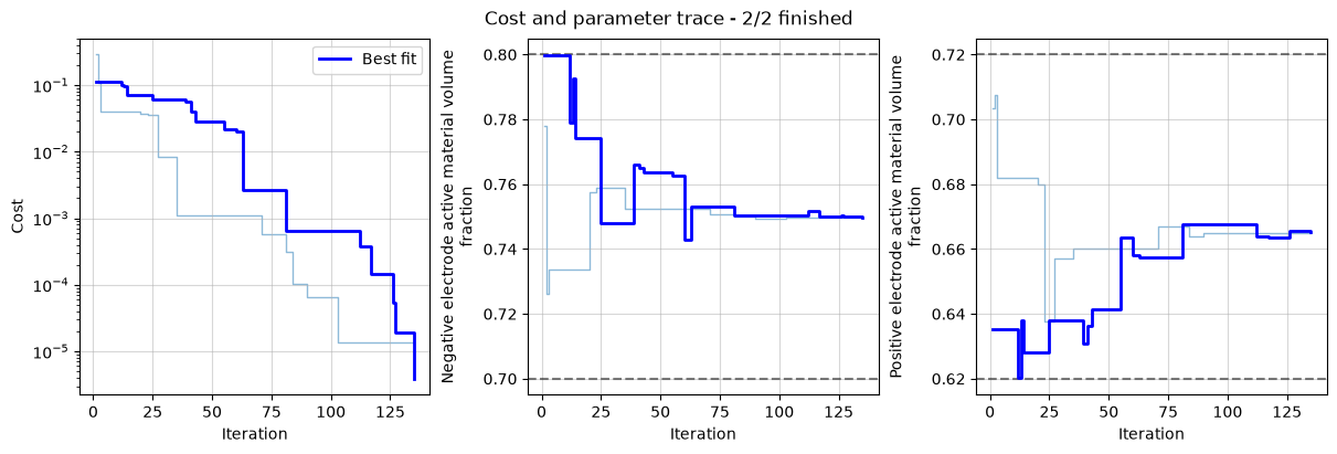
Each line is tagged with the start that produced it, so the two starts above interleave as they progress. The sink runs on the driver, so this output is identical whether the fit runs on one worker or fifty — which is exactly what a print in an objective cannot give you.

The sink only decides where progress is shown. The fit records its own trace whichever sink you pass, which is why plot_trace() works above.

For an ArrayDataFit, each line also names its element — [25.0:0] is start 0 of the element at 25.0 — since every element restarts its start ids from "0". To show your own names instead, pass labels; one is used per element, in run order, including an element that is canceled before any start finishes:

PrintSink(labels=[f"{T} K" for T in temperatures])

A sink is also the place to send progress somewhere other than the terminal — implement emit(event) and pass it as progress_sink to record generations to a file, a database, or a live plot. Its last event for each fit is an ExecutionFinished, delivered however the fit ended.

Objective-level parallelism

tasks_per_point was 3 because the three objectives were dispatched separately. That is the default for a multi-objective fit, and it multiplies the width of every generation. It is set on the DataFit rather than the ExecutionConfig, because whether objectives can be split depends on the cost function, not on the machine.

Turning it off batches all of a point’s objectives into one task: fewer, larger tasks and a narrower fit. That is the right trade when the objectives are cheap enough that per-task overhead dominates.

for mode in ("auto", "off"):
    fit = iwp.DataFit(
        objectives,
        parameters=parameters,
        multistarts=4,
        options={"seed": 0},
        optimizer=iwp.optimizers.CMAES(population_size=8, max_iterations=15),
        objective_parallelism=mode,
    )
    fit.setup(known_parameters)
    print(
        f"objective_parallelism={mode!r:>7}: "
        f"tasks_per_point={fit.tasks_per_point()}, "
        f"max_useful_workers={fit.max_useful_workers()}"
    )

objective_parallelism= 'auto': tasks_per_point=3, max_useful_workers=96
objective_parallelism=  'off': tasks_per_point=1, max_useful_workers=32

Summary

• ExecutionConfig(num_workers=N) is the one setting for local pool size.

• The pool is min(max_useful_workers(), N); check max_useful_workers() before asking for more. For a population optimizer that ceiling is multistarts x population_size x tasks_per_point.

• A pool pays off only when the warm evaluation cost is large relative to the per-worker model build. Measure both before scaling up.

• Watch progress with progress_sink=PrintSink(); a print inside an objective runs in a worker and is discarded.

• num_workers=1 skips the pool entirely and runs in-process, which is the easiest way to debug an objective that raises.